• 1. Introduction
    • 1.1 The main problem
    • 1.2 Objective
    • 1.3 Specific objectives
    • 1.4 What is snoRNA?
    • 1.5 Machine Learning
    • 1.6 Feature Extraction
    • 1.7 Evaluation Metrics
  • 2. Methodology
    • 2.1 Search strategy
    • 2.2 Inclusion and exclusion criteria
  • 3. Project Pipeline
    • 3.1 Step 1: Collect Data
    • 3.2 Step 2: Data preprocessing
    • 3.3 Step 3: Extraction
    • 3.4 Step 4: Training and Testing
    • 3.5 Step 5: Evaluation
  • 4. Evaluation
    • 4.1 Statistics
    • 4.2 Study Case

Feature extraction in snoRNAs using mathematical approach

Graduation project to Bachelor's degree in Computer Science.

The graduation project aims to analyze mathematical models of feature extraction such as the Fourier method, Entropy and Complex Networks in the classification of C/D box and H/ACA box snoRNAs in vertebrate and invertebrate organisms.

The main problem

The search for Machine Learning (ML) techniques capable of identifying the characteristics of secondary structures of RNAs has become fundamental over the last few years due to the large amount of data on genetic content.

Traditional ML feature extraction methods are not always able to determine an effective model that can avoid the loss of information from the structure, a good example are the snoRNA classes.

Objective

Therefore, the objective of the work is to guarantee an effective extraction method for classifying snoRNA classes. The main idea is to show that mathematical methods, despite being general, are good enough as biological methods to classify the two classes of snoRNAs: H/ACA box and C/D box

Specific objectives

  1. Collect and process snoRNA data to create a set of training and testing data;
  2. Use a feature extraction algorithm with a mathematical approach such as Fourier transform, numerical mapping, entropy (Shannon and Tsallis), networks complex, EDeN and/or etc;
  3. Extract features from mathematical models of both classes of snoRNAs (H/ACA box and C/D box);
  1. What is a snoRNA?
  2. SnoRNAs are one of the oldest and most numerous families of non-coding RNAs (ncRNAs), are widely present in the nucleoli of eukaryotic cells and are 60–300 nt long. The main function of snoRNAs is to guide the modification of ribosomal RNA site-specific (rRNA).

    SnoRNAs are mainly encoded by intronic regions of coding genes protein and non-protein coding. Typically, they can be classified into two groups: H/ACA box and C/D box.

    snoRNA C/D box
    Secondary structure of SNORD33, which belongs to the C/D box group. Extracted image by RFAM
    snoRNA H/ACA box
    Secondary structure of SNORA26, which belongs to the H/ACA box group. Image extracted from RFAM
  3. Machine Learning
  4. Machine Learning is a branch of artificial intelligence that involves constant self-learning algorithms to perform classification and regression tasks. Given a set of data, the algorithm will train based on predefined features that describe the snoRNA.

    The initial hypothesis is that there is a function f that manage to be applicable to a group X of the genetic code that characterizes it as an snoRNA C/D box or H/ACA box.

    ML Workflow
    Machine Learning Workflow

    The Machine Learning workflow can be divided into 5 steps:

    1. Data gathering: The first step in the process of machine learning is to obtain authentic data to construct the set positive and negative, and can be acquired from existing databases or from online repositories, as long as it is from a reliable source.

    2. Data preprocessing: This step is crucial in the flow of ML to work and also the one that takes the most time. The data may be in any format so it had to be converted to a standard format. Therefore, it is essential to check whether the amount of data for the sets (positive and negative) are balanced, if the genetic sequences holds similar sizes, if the genome contains only nitrogenous bases, and so on.

    3. Feature Extraction: Feature extraction refers to the process of transformation of raw data into numerical data that can be processed, preserving the information in the original dataset. It is a fundamental step, because the machine learning algorithm produces better results with values continuous and discrete data than directly with raw data.

    4. Training: An ML algorithm is aplied on the data set of training with the aim of learning and predicting certain "behaviors" based in the real values ​​arising from the extraction. These algorithms can fall into three major categories: binary, classification and regression. In this work, the classification algorithm.

    5. Test: Once the model is trained exhaustively, the next step is to test it and validate it to ensure it is effective. Using the obtained test dataset in the previous step, the accuracy of the obtained model is checked and validated.
  5. Feature Extraction
  6. Feature extraction is a part of the dimensionality reduction process, in which an initial set of raw data is divided and reduced into more manageable groups so that reduce the complexity of the processing phase. The most important characteristic of these large data sets is that they have a large number of variables. These variables require a lot of computing resources to be processed, therefore, extracting features helps you get the best feature from these big data sets by selecting and combining variables, effectively reducing the amount of data. These features are transcribed into numerical values ​​capable of describing the real data set accurately and originaly

    There are many feature extraction techniques, however, the focus of this work is to analyze the procedures that use mathematical concepts to extract attributes (features) from the set of data. Therefore, the project will be responsible for explaining the operation of 3 extraction algorithms: Numerical Fourier Transformation, Entropy and Complex Networks.

  7. Evaluation metrics
  8. To check whether the classifier was able to correctly predict the set training, you need to measure your ability to predict the model. The accuracy of classification is used to measure model performance, however, the evaluation will not always be satisfactory and the results will vary according to the chosen metric. There are metrics such as Precision, Recall, F1, F-Beta and Roc-AUC, and, in general, the matrix of Confusion is the basis of calculation for these metrics.

    Those metrics will be demonstrated on metholodogy section.

    ML Workflow
    How a confusion matrix works. Extracted from datacamp

Search strategy

Databases like PubMed Central, UnB repository, Oxford Academic, Medline, SIABI/IFB were consumed for theoretical and argumentative basis of the work

Database consumed
Database URL
PubMed Central https://pubmed.ncbi.nlm.nih.gov
UnB Repository https://repositorio.unb.br
Oxford Academic https://academic.oup.com/journals
Medline http://bases.bireme.br/
SIABI/IFB http://siabi.ifb.edu.br/

For each database chosen, advanced searches were carried out in their tools of research with a time interval of 6 years until the date of this review (24 June 2022), including research keywords: ncRNAs, machine learning, feature extraction, sequence features, mathematical approach which resulted in a set of more than 300 literatures

Result of database searches
Database Keywords Scientific Projects
PubMed Central Machine learning, sequence features, ncRNAs 98
UnB Repository Machine learning, ncRNAs 5
Oxford Academic Machine learning, ncRNAs, mathematic sequence features 153
Medline Machine learning, ncRNAs, mathematic sequence 34
SIABI/IFB Machine learning 2

Inclusion and exclusion criteria

  1. Inclusion criteria (IC1): Scientific productions that use ncRNAs as an object search for feature extraction;
  2. Inclusion criteria (IC2): Primary studies that apply supervised or unsupervised predictive models, whether biological, hybrid or mathematical, to classify ncRNAs;
  3. Inclusion criteria (IC3): Studies that classify classes and groups of ncRNAs applying the model feature extraction mathematician;

Exclusion Criteria (EC) will help filter only relevant scientific articles for review. Based on the research questions that guide the work, the CEs proposed below select a concrete group of productions in order to reduce the scope and generalization of the topic.

  • Studies that are not written in Portuguese or English;
  • Studies which the full version is not available free of charge;
  • "Duplicate" studies, which were obtained by searching more than one database, in these cases only the first will be considered.
  • Scientific productions that do not classify the group of ncRNAs;
  • Descriptive studies of functionalities that do not discuss the methodology of Machine learning (ML) employed;

Step 1: Collect data


Positive sample

First, to gather data to collect all the snoRNAs C/D box and H/ACA box samples, the RFAM database will be used as reference to get all the families of each snoRNA class. In their current webpage, it has an API reference to connect to the MYSQL database with the user rfamro with host mysql-rfam-public.ebi.ac.uk

                
                    mysql --user rfamro --host mysql-rfam-public.ebi.ac.uk --port 4497 --database Rfam
                    SHOW DATABASES;
                    USE family;
                    SHOW TABLES;
                    SELECT rfam_id, type, description FROM family WHERE type LIKE '%snoRNA%';


The idea is to get the RFAM_ID to get the fasta format file to use the genetic content of nitrogenous bases as characteristics of the family. The query it will only accept snoRNAs of class C/D box and H/ACA box, so it is necessary to filter the TYPE column and output that query to a file specified by the class itself.

SELECT rfam_id FROM family WHERE type like '%snoRNA; CD-box%' INTO OUTFILE 'cd-box'; SELECT rfam_id FROM family WHERE type like '%snoRNA; HACA-box%' INTO OUTFILE 'haca-box';

Remember that this families are the positives samples for the classifier. The negative sample will be explained how it was built and how it managed to deal with overfitting issues.

A simple shell script was created to automatically download all sequences of each family from the RFAM FTP Site Directory, defining the file name based on the rfam_id name with the format of the fasta extension, which is the standard extension format representation of nucleotide sequences. Each file was assigned to the folder with the name of your snoRNA class inside the positives folder.

for $file in $(ls positives/); do curl http://http.ebi.ac.uk/pub/databases/Rfam/CURRENT/fasta_files/$file.fa.gz -O; done; for $file in $(ls fasta/); do gzip -d $file.gz; done;

In total, 4877 C/D box snoRNA sequences were obtained from 475 families and 2813 H/ACA box snoRNA sequences among 283 families for the positive set of data.

Negative sample

It is necessary the negative set to train and test the classification model to be generated, then, the elaboration of the negative set had as a fundamental rule that 50% of the set would be created by sequences generated randomly by a shuffling as the other half would be formed by genetic sequences of RNAs such as Ribonuclease (RNase) P, 5S ribosomal RNA (rRNA) and transfer RNA (tRNA), considering that the maximum size delimited for the negative set would be three times larger than the positive set. The same idea aplied before was used here: gathering data from MYSQL RFAM database, save the output to a file and them make requests calls to RFAM FTP Site to get the fasta content of each RFAM_ID.

The effort to build the negative set not only used differente RNAs classes but an shuffle algorithm was implement providing a total of 4999 sequences, 2433 of which were RNA sequences not belonging to snoRNAs and 2566 random sequences.

                
                    # A simple shuffle algorithm
                    # It mix up the nitrogenous bases to create random genetic sequences.
                    def shuffle(sequence, times, order):
                        seq = sequence
                        sequences = []
                        for i in range(times):
                            kmers = [seq[i:i + order] for i in range(0, len(seq), order)]
                            random.shuffle(kmers)
                            seq_out = ''.join(kmers)
                            sequences.append(seq_out)
                        return sequences


Step 2: Data preprocessing

Using the families as a basis for calculation and construction of the positive set, the 85% percentile of the data, the arithmetic mean, the variance, and the maximum and minimum value of the quantities of sequences as expressed in the table below.

Positive Dataset Metrics.
Class Sequences Families Percentile Mean Variance Max Min
C/D box 4877 475 6 4 2.5589 7 2
H/ACA box 2813 283 22 5 27884.03 76 2

The calculation metrics are balanced through the arithmetic mean and the number of expected sequences per family so that the machine learning algorithm consumes them in equivalent grouping. Thus, when presetting this condition, 1553 sequences remained of C/D box and 1013 H/ACA box sequences to compose the positive dataset.

According to the pre-established condition in the negative dataset, 1500 randomly generated sequences were obtained and 1666 sequences made up of the mixture of RNase P, 5S rRNA and tRNA, totaling 3166 sequences in the negative dataset.

Step 3: Extraction

The feature extraction methods used are mathematical in nature as the numerical mapping with the Fourier transformations (Real, Z-curve), the entropies of Shannon and Tsallis and complex networks. All feature extraction algorithms can be extracted from BONIDIA et. al. (2021)

The creation of scripts in the extraction stage was essential for automating activities repetitive tasks in terms of efficiency and speed as it facilitated the adjustment of parameters for the extraction algorithms, the organization of data input and output into files (mainly to those that contained the fasta format in their extension) and the parallel execution of the algorithms to speed up the data extraction and grouping phase.

                
                    # A bash script that verify what extraction method the user
                    # passes as argument.
                    extract() {
                        local group=$1
                        local method=$2
                        local fourier_number=$3
                        local entropy_choice=$3
                        local algorithm
                        local output_directory
                        case $method in
                        "complex")
                            if [ $group = 'cdbox' ]; then
                                for file in $CD_BOX_DIRECTORY; do
                                    archive=$(echo -e $file | cut -f3 -d "/" | cut -f1 -d ".")
                                    python3 $COMPLEX_ALGORITHM -i $file -o $OUTPUT_CDBOX_EXTRACT_COMPLEX_DIRECTORY/$archive.csv -l cdbox -k 3 -t 10 1>/dev/null
                                    echo -e "Negative sample\t$group\t$method\t$archive.csv\n"
                                done
                            elif [ $group = 'hacabox' ]; then
                                for file in $HACA_BOX_DIRECTORY; do
                                    archive=$(echo -e $file | cut -f3 -d "/" | cut -f1 -d ".")
                                    python3 $COMPLEX_ALGORITHM -i $file -o $OUTPUT_HACABOX_EXTRACT_COMPLEX_DIRECTORY/$archive.csv -l hacabox -k 3 -t 10 1>/dev/null
                                    echo -e "Extracting...\t$group\t$method\t$archive.csv"
                                done
                            elif [ $group = 'negative' ]; then
                                archive="negative_complex"
                                python3 $COMPLEX_ALGORITHM -i $NEGATIVE_FILE -o $OUTPUT_CDBOX_NEGATIVE_EXTRACT_COMPLEX_DIRECTORY/$archive.csv -l negative -k 3 -t 10 1>/dev/null
                                python3 $COMPLEX_ALGORITHM -i $NEGATIVE_FILE -o $OUTPUT_HACABOX_NEGATIVE_EXTRACT_COMPLEX_DIRECTORY/$archive.csv -l negative -k 3 -t 10 1>/dev/null
                                echo -e "$group\t$method\t$archive.csv"
                            elif [ $group = 'real' ]; then
                                for file in $REAL_DATA_DIRECTORY; do
                                    archive=$(echo -e $file | cut -f3 -d "/" | cut -f1 -d ".")
                                    python3 $COMPLEX_ALGORITHM -i $file -o $OUTPUT_REAL_DATA_COMPLEX_DIRECTORY/$archive.csv -l real -k 3 -t 10 1>/dev/null
                                    echo -e "Extracting...\t$group\t$method\t$archive.csv"
                                done
                            else
                                echo -e "Unrecognized group of snoRNAs."
                                exit 0
                            fi
                            ;;
                        # ...
                    }


The extraction returned a file in csv format covering the columns with the characteristics found in each family by the algorithms. It is worth noting that these data are purely continuous, therefore, it is possible for there to be infinite values ​​that are not numeric. It is important to have the awareness of this property of the data because later there will be a treatment around these values ​​in the classifier pre-execution stage.

Step 4: Training and Testing

The training and testing set was divided such that 70% of the original set was for training while the remaining 30% remained for the test set and these values ​​were passed to the train_test_split function provided by the sklearn.model_selection package in Python. In training without cross-validation, there is a parameter called test_size responsible for establish the number of iterations that the training algorithm will perform so that in the end it can evaluate which of these output models had the best benefit. On the other hand, in training with cross-validation, the n_estimators parameter designates the proportion of models in a single execution of the algorithm in order to obtain the best estimator among the evaluated portion supported by evaluation metrics.

The Random Forest classification algorithm was chosen because it was a promising algorithm in literary review whose generalization was tested in different classification tasks for long non-coding RNAs (lncRNAs) from unbalanced data.

                
                    class snoRNAs():
                        # ...
                        def train(self):
                            for key, value in self.extraction_methods.items():
                                for _ in range(self.test_counter):
                                    initial_time = time.time()
                                    X, y = value.get_XY()
                                    X_train, X_test, y_train, y_test = train_test_split(X, y, test_size=0.3)
                                    clf = RandomForestClassifier(max_depth=10)
                                    clf.fit(X_train, y_train)
                                    predictions = clf.predict(X_test)
                                    self.evaluation.append((value.group, value.method, clf, f1_score(y_test, predictions), y_test))
                                    plot_graph(value, y_test, predictions, self.cm_arr)
                                    self.f1_scores.append(str(f1_score(y_test, predictions) * 100.0) + "%")
                                    self.fbeta_scores.append(
                                        str(fbeta_score(y_test, predictions, beta=0.5) * 100.0) + "%"
                                    )
                                    self.recalls.append(str(recall_score(y_test, predictions) * 100.0) + "%")
                                    self.precisions.append(
                                        str(precision_score(y_test, predictions, average="macro") * 100.0) + "%"
                                    )
                                    self.auc.append(str(roc_auc_score(y_test, predictions) * 100.0) + "%")
                                    self.labels.append(value.group)
                                    self.methods.append(key)
                                    end_time = time.time()
                                    self.measure_time.append(str(end_time - initial_time) + "s")
                                    group, method, clf, y_test = self._evaluate_model(self.evaluation)
                                    model_file = f"{group}_{method}_{self.datetime_str}.pickle"
                                    save_model(model_file, clf)
                                    self.test(y_test, model_file, group, method)
                                    self.evaluation.clear()
                                    deviation = dp(self.cm_arr)
                                    avg = average(self.cm_arr)
                                    self.standard_deviations.append(
                                        {"class": value.group, "method": value.method, "deviation": deviation}
                                    )
                                    self.averages.append({"class": value.group, "method": value.method, "average": avg})
                        def test(self, y_test, model_file, group, method):
                            path = f'./models/{model_file}'
                            model = load_model(path)
                            real_valid = CSVData(group, method)
                            out_file = f"./output/validation/validation_{self.datetime_str}.csv"
                            content = ""
                            if not path.isfile(out_file):
                                content = f'classe,metodo,organismo,positivos,negativos,total,modelo,eficiencia\n'
                                f = open(out_file, "w")
                            else:
                                f = open(out_file, "a+")
                                for org in self.list_organisms_real_data:
                                    X = real_valid.get_X(org)
                                    prediction = model.predict(X)
                                    pos = 0
                                    neg = 0
                                    total = 0
                                    for i in prediction:
                                        if i == 1:
                                            pos += 1
                                        else:
                                            neg += 1
                                        total = pos + neg
                                        content += f'{group},{method},{org},{pos},{neg},{total},{model_file},{pos/total}\n'
                                    f.write(content)
                                    f.close()


The tuning hyper-parameters used in Random Forest for each extraction method characteristics are shown in the table below:

Random Forest Hyperparameters without using the GridSearchCV function.
Parameters Value
"bootstrap" true
"ccp_alpha" 0.0
"class_weight" None
"criterion" gini
"max_depth" 10
"max_features" sqrt
"max_leaf_nodes" None
"max_samples" None
"min_impurity_decrease" 0.0
"min_samples_leaf" 1
"min_samples_split" 2
"min_weight_fraction_leaf" 0.0
"n_estimators" 100
"n_jobs" None
"oob_score" false
"random_state" None
"verbose" 0
"warm_start" false

To automate this hyperparameter tuning process, the function GridSearchCV from the sklearn module in Python. The primary objective of GridSearchCV is to create of parameter combinations from an exhaustive search over specified values ​for an estimator (score, that is, evaluation metric), to later evaluate them. The estimator parameters used to apply these methods are optimized and refined by cross-validation over a grid of parameters.

                
                    class snoRNAs():
                        # ...
                        def train_with_cv(self):
                            space = dict()
                            space['n_estimators'] = [10, 100, 500]
                            for key, value in self.extraction_methods.items():
                                initial_time = time.time()
                                X, y = value.get_XY()
                                X_train, X_test, y_train, y_test = train_test_split(X, y, test_size=0.3)
                                model = RandomForestClassifier(max_depth=10)
                                clf_f1 = GridSearchCV(model, space, scoring="f1", refit=True)
                                clf_precision = GridSearchCV(model, space, scoring="precision", refit=True)
                                clf_recall = GridSearchCV(model, space, scoring="recall", refit=True)
                                clf_accuracy = GridSearchCV(model, space, scoring="accuracy", refit=True)
                                clf_auc = GridSearchCV(model, space, scoring="roc_auc", refit=True)
                                result_f1 = clf_f1.fit(X_train, y_train)
                                result_precision = clf_precision.fit(X_train, y_train)
                                result_recall = clf_recall.fit(X_train, y_train)
                                result_accuracy = clf_accuracy.fit(X_train, y_train)
                                result_auc = clf_auc.fit(X_train, y_train)
                                self.test_with_cv(result_f1.best_estimator_, result_f1.best_score_, "f1", value.group, value.method)
                                self.test_with_cv(result_precision.best_estimator_, result_precision.best_score_, "precision", value.group, value.method)
                                self.test_with_cv(result_recall.best_estimator_, result_recall.best_score_, "recall", value.group, value.method)
                                self.test_with_cv(result_accuracy.best_estimator_, result_accuracy.best_score_, "accuracy", value.group, value.method)
                                self.test_with_cv(result_auc.best_estimator_, result_auc.best_score_, "auc_roc", value.group, value.method)
                                predictions = clf_f1.predict(X_test)
                                plot_graph(value, y_test, predictions, self.cm_arr)
                                self.f1_scores.append(str(f1_score(y_test, predictions) * 100.0) + "%")
                                self.fbeta_scores.append(
                                        str(fbeta_score(y_test, predictions, beta=0.5) * 100.0) + "%"
                                    )
                                self.recalls.append(str(recall_score(y_test, predictions) * 100.0) + "%")
                                self.precisions.append(
                                        str(precision_score(y_test, predictions, average="macro") * 100.0) + "%"
                                    )
                                self.auc.append(str(roc_auc_score(y_test, predictions) * 100.0) + "%")
                                self.labels.append(value.group)
                                self.methods.append(key)
                                end_time = time.time()
                                self.measure_time.append(str(end_time - initial_time) + "s")
                        def test_with_cv(self, best_model, best_score, score_type, group, method):
                            real_valid = CSVData(group, method)
                            out_file = f"./output/validation/{score_type}_{self.datetime_str}.csv"
                            content = ""
                            if not path.isfile(out_file):
                                content = f'classe,metodo,organismo,positivos,negativos,total,eficiencia,{score_type}\n'
                                f = open(out_file, "w")
                            else:
                                f = open(out_file, "a+")
                            for org in self.list_organisms_real_data:
                                X = real_valid.get_X(org)
                                prediction = best_model.predict(X)
                                pos = 0
                                neg = 0
                                total = 0
                                for i in prediction:
                                    if i == 1:
                                        pos += 1
                                    else:
                                        neg += 1
                                total = pos + neg
                                content += f'{group},{method},{org},{pos},{neg},{total},{pos/total},{best_score}\n'
                            f.write(content)
                            f.close()


Similar to Random Forest's default hyperparameters, GridSearchCV applied the following parameters as shown in the table below:

Random Forest hyperparameters after using the GridSearchCV function.
Parameters Value
"mean_fit_time" array([0.03470263, 0.34155726, 1.70107441])
"std_fit_time" array([0.00415981, 0.02498759, 0.14168099])
"mean_score_time" array([0.00217724, 0.01229601, 0.04444399])
"std_score_time" array([0.0001098 , 0.00510206, 0.01017052])
"param_n_estimators" masked_array(data=[10, 100, 500])
"mask" array([False, False, False])
"params" array([’n_estimators’: 10, ’n_estimators’: 100, ’n_estimators’: 500])
"split0_test_score" array([0.98817967, 0.99061033, 0.99061033])
"split1_test_score" array([0.98337292, 0.98329356, 0.98337292])
"split2_test_score" array([0.98584906, 0.98352941, 0.98352941])
"split3_test_score" array([0.98345154, 0.98113208, 0.98113208])
"split4_test_score" array([0.98578199, 0.98584906, 0.98578199])
"mean_test_score" array([0.98532703, 0.98488289, 0.98488535])
"std_test_score" array([0.00178623, 0.00322997, 0.00321846])
"rank_test_score" array([1, 3, 2])

Step 5: Evalutation


Case studies: classification of snoRNAs in a dataset found in literature

In the case studies, the operations were divided into N executions and for each execution evaluation metrics will be checked so that in the testing stage the best model found for each extraction method.

Training validations involve any validation the model needs be retrained. Typically, this includes testing different models during a single pipeline. training. These validations are performed in this training/evaluation phase of model development, and are often kept as experimentation code, not doing anything else. part of the final product of the classifier.

The training pipeline starts when loading the predictive model with the best accuracy on the f1_score score by feature extraction method, two case studies are then done around the real world dataset like the genome of vertebrates and invertebrates such such as chickens, flies belonging to the Drosophilidae family, Nematodes from the Rhabditidae family, protozoa of the Trypanosomatidae family such as Leishmania, Homo Sapiens and Platypuses:

  • Case Study 1: Add the real dataset according to its respective class of snoRNAs from the genomes found and use the model to predict this set.
  • Case Study 2: Compare the results obtained by predicting the set of training by evaluating classifier behavior with references from others articles that predicted the two classes of snoRNAs (C/D box and H/ACA box)

Before estimating the predictive model, in case studies in which a cross validation, the training run divides the set into training and testing data in different parts of the model in a way that validates the performance of each model on a given interval, ensuring the generalization of the data presented among the best parameters found.

The calculation of hits and errors is done using the confusion matrix that shows the frequencies classification for each class of snoRNAs. The matrix leads us to a brief analysis of the estimates even if it has not been included in an evaluation metric.

Confusion Matrix of Shannon's Entropy
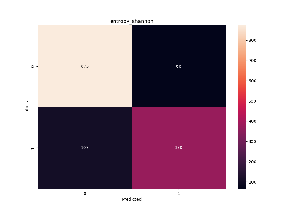
Confusion matrix in the training stage using the Shannon Entropy method for the C/D box class of snoRNAs.

Which can be interpreted and created by code as follow:

                
                    def get_cm(obj, y_test, predictions, tp_arr):
                        cm = confusion_matrix(y_test, predictions)
                        tn, fp, fn, tp = cm.ravel()
                        tp_arr.append(
                            {
                                "class": obj.group,
                                "method": obj.method,
                                "tn": tn,
                                "fp": fp,
                                "fn": fn,
                                "tp": tp,
                            }
                        )
                        print(f"{COLORS.BOLD}[DEBUG] {COLORS.SUCCESS}{obj.group}\t{obj.method}\t{cm.ravel()}{COLORS.ENDC}")
                        return cm


Statistics

To identify H/ACA box and C/D snoRNAs, two datasets were constructed different for each class of snoRNAs. For the learning phases, a set of data as training and the other for testing using the hold-out method of separation and cross validation respectively. Each training was repeated 10 times, and the calculation of metrics, standard deviation and mean are displayed in the tables for each snoRNA class and extraction method used. It is extremely important to know that these metrics were extracted of the best estimators, that is, the best model found based on the f1_score in around the training involved.

Test phase results for C/D box snoRNAs: F-score (FSC), Accuracy (Acc), Recall (REC), Average Precision (PRE), Area under the ROC curve (AUC). The mean and standard deviation total of each metric.
snoRNAs Class Extraction Method FSC (%) ACC (%) REC (%) PRE (%) AUC (%)
C/D box Fourier Real 98.25 98.81 97.26 99.18 99.85
C/D box Fourier Z-Curve 98.81 99.15 98.27 99.35 99.96
C/D box Shannon's Entropy 79.83 87.37 76.47 84.01 93.71
C/D box Tsallis's Entropy 79.34 86.58 78.34 80.09 93.35
C/D box Complex Networks 99.72 99.79 99.53 99.94 99.98
Mean (%) 90.70 94.35 89.97 92.51 97.37
Standard Deviation (%) 10.60 6.73 11.52 9.65 2.72
Test phase results for H/ACA box snoRNAs: F-score (FSC), Accuracy (Acc), Recall (REC), Average Precision (PRE), Area under the ROC curve (AUC).
snoRNAs Class Extraction Method FSC (%) ACC (%) REC (%) PRE (%) AUC (%)
H/ACA box Fourier Real 98.25 98.81 97.26 99.18 99.85
H/ACA box Fourier Z-Curve 98.81 99.15 98.27 99.35 99.96
H/ACA box Shannon's Entropy 79.83 87.37 76.47 84.01 93.71
H/ACA box Tsallis's Entropy 79.34 86.58 78.34 80.09 93.35
H/ACA box Complex Networks 99.72 99.79 99.53 99.94 99.98
Mean (%) 90.70 94.35 89.97 92.51 97.37
Standard Deviation (%) 10.60 6.73 11.52 9.65 2.72

Study Case

To validate the Random Forest classifier using mathematical methods, we used the concepts of cross validation to separate each k-fold or k-part where the value of k = 5. For each fold, both sets were separated and the desired metrics (F1, AUC, PRE, REC, ACC). According to the best estimator, the model was chosen and separated for that is evaluated on a real dataset with predicted vertebrate sequences and invertebrates, some of these organisms have been partially confirmed in experiments in humans, nematodes, drosophilids, platypuses, chickens and leishmania.

Comparing the results obtained in ARAUJO (2017) by snoReport 2.0 taking into account counts the validation sets of the cited articles, tables 5.10 show how effective the predictor in classifying snoRNAs into C/D box or H/ACA box, using as a comparative basis the work mentioned below.

Results obtained in the work of ARAUJO (2017) using the snoReport 2.0 software on the classes of snoRNAs.
Set C/D H/ACA
Homo Sapiens (21/21) (28/32)
Platypus (42/144) (45/73)
Gallus gallus (112/132) (66/69)
Nematodes (32/108) (46/60)
Drosophila (2/63) (39/56)
Leishmania (0/62) (0/37)
Real Fourier Method.
Set C/D H/ACA
Homo Sapiens (21/21) (28/33)
Platypus (143/144) (69/73)
Gallus gallus (124/132) (67/69)
Nematodes (106/108) (60/60)
Drosophila (63/63) (55/56)
Leishmania (54/62) (36/37)
Fourier Z-Curve Method.
Set C/D H/ACA
Homo Sapiens (21/21) (33/33)
Platypus (144/144) (72/73)
Gallus gallus (125/132) (69/69)
Nematodes (106/108) (59/60)
Drosophila (63/63) (55/56)
Leishmania (61/62) (36/37)
Shannon Entropy Method.
Set C/D H/ACA
Homo Sapiens (21/21) (18/33)
Platypus (128/144) (30/73)
Gallus gallus (109/132) (24/69)
Nematodes (73/108) (13/60)
Drosophila (46/63) (8/56)
Leishmania (45/62) (17/37)
Tsallis Entropy Method.
Set C/D H/ACA
Homo Sapiens (19/21) (27/33)
Platypus (127/144) (52/73)
Gallus gallus (114/132) (24/69)
Nematodes (83/108) (17/60)
Drosophila (49/63) (30/56)
Leishmania (54/62) (21/37)
Complex Networks Method.
Set C/D H/ACA
Homo Sapiens (21/21) (33/33)
Platypus (144/144) (73/73)
Gallus gallus (127/132) (69/69)
Nematodes (107/108) (60/60)
Drosophila (62/63) (56/56)
Leishmania (61/62) (37/37)

Separately, in summary, the classifier was efficient in identifying the organisms vertebrates and invertebrates from the validation set. Considering that the total number of sequences of the snoRNAs C/D box class of vertebrate organisms is 297 and invertebrates is 233 and for the of the snoRNAs class H/ACA box is 175 and 153 respectively, it is evident that the algorithms Fourier and Complex Networks were considerably significant in the classification, having an accuracy greater than 90% in both predictions of the two classes of snoRNAs. Even though the Entropy methods were not as efficient, for the C/D box snoRNAs class they managed to have an efficiency of around 80% accuracy.

The following tables show the diagnosis of the number of sequences found by the feature extraction method in vertebrate and invertebrate organisms in comparison with the work of ARAUJO (2017).

Number of sequences found using snoReport 2.0 in the research work of ARAUJO (2017).
Tool C/D Accuracy (C/D) H/ACA Accuracy (H/ACA)
snoReport 2.0 (vertebrate) 175 58.92 139 79.88
snoReport 2.0 (invertebrate) 34 14.59 85 55.55
Number of sequences found by feature extraction method in vertebrate organisms.
Method C/D Accuracy (C/D) H/ACA Accuracy (H/ACA)
Real Fourier 288 96.96 161 96.56
Z-Curve Fourier 291 97.97 174 99.14
Shannon Entropy 250 84.17 84 67.38
Tsallis Entropy 255 85.85 128 77.58
Complex Networks 292 98.31 175 98.71
Number of sequences found by feature extraction method in invertebrate organisms.
Method C/D Accuracy (C/D) H/ACA Accuracy (H/ACA)
Real Fourier 225 92.0 150 98.03
Z-Curve Fourier 231 99.42 150 98.03
Shannon Entropy 157 48.0 65 42.48
Tsallis Entropy 181 73.14 88 57.51
Complex Networks 230 100.0 152 99.34